Estimating directional spectra from ADCP data

This example show how to compute the wavelet-based directional wave spectra from bottom-mounted ADCP (Acoustic Doppler Current Profilers) data using different approaches. First, as ADCP usually have 3 to 5 (sometimes more) slanted acoustic beams, the surface elevation at different spatial points can be extracted. This is done considering that the acoustic backscatter is maximum when is reflected by the sea surface. The spatial array is then constructed projecting the beam geometry onto the sea surface. The second approach consider the triplet formed by the horizontal components of the wave-induced velocty and the echo-based surface elevation from the vertical beam (see Pelaez-Zapata et al. 2024 for more details.)

import numpy as np
import xarray as xr

from matplotlib import pyplot as plt

import ewdm
from ewdm.plots import plot_directional_spectrum

Exploring ADCP dataset

As you can see, the typical ADCP data contains echo-based sea surface elevation at each acoustic beam so we can try to compute the directional spectrum using our ewdm.Arrays approach, but also we see the three velocty components, which means that we can also compute the directional spectra using our ewdm.Triplets approach.

adcp_dataset = xr.open_dataset("../../data/adcp_test_data.nc")
print(adcp_dataset)

<xarray.Dataset> Size: 2MB
Dimensions:   (beam: 5, time: 3720, cell: 38)
Coordinates:
  * time      (time) datetime64[ns] 30kB 2017-02-23 ... 2017-02-23T00:30:59.5...
  * cell      (cell) int32 152B 1 2 3 4 5 6 7 8 9 ... 30 31 32 33 34 35 36 37 38
  * beam      (beam) int32 20B 1 2 3 4 5
Data variables:
    eta       (beam, time) float32 74kB ...
    vel_x     (cell, time) float32 565kB ...
    vel_y     (cell, time) float32 565kB ...
    vel_z     (cell, time) float32 565kB ...
    pressure  (time) float32 15kB ...
    z_cell    (cell) float32 152B ...
Attributes:
    title:                   ADCP deployment winter 2016/2017 coast off of In...
    summary:                 ADCP deployment winter 2016/2017 coast off of In...
    latitude:                53.0671
    longitude:               -9.6266
    institution:             UCD Wave Group
    date_created:            2020-09-16
    convention:              CF-1.8
    keywords:                adcp, ocean currents, sea_surface_waves, aran_is...
    platform:                ADCP Teledyne RDI Sentinel V
    creator:                 Daniel Pelaez-Zapata
    principal_investigator:  Frederic Dias

water_depth = adcp_dataset["pressure"].mean("time").item()
print(f"The total water depth is {water_depth:.2f} m")
print(f"The number of vertical cells is: {len(adcp_dataset['cell'])}")
print(f"The number acoustic beams is: {len(adcp_dataset['beam'])}")

The total water depth is 46.09 m
The number of vertical cells is: 38
The number acoustic beams is: 5

Triplets approach

Let’s first try the triplets approach as it is more direct.

norm = lambda x: x - np.nanmean(x)

time = adcp_dataset["time"].data
surface_elevation = norm(adcp_dataset["eta"].sel(beam=5).data)

fig, ax = plt.subplots(1, 3, figsize=(8,3), layout="constrained")
for i, cell in enumerate([5, 10, 20]):

    cell_depth = water_depth-adcp_dataset["z_cell"].isel(cell=cell).item()

    eastward_velocity = norm(adcp_dataset["vel_x"].isel(cell=cell).data)
    northward_velocity = norm(adcp_dataset["vel_y"].isel(cell=cell).data)

    spec = ewdm.Triplets.from_numpy(
        time = time,
        surface_elevation = surface_elevation,
        eastward_velocity = eastward_velocity,
        northward_velocity = northward_velocity,
    )

    output_triplets = spec.compute(use="velocities")

    plot_directional_spectrum(
        output_triplets.directional_spectrum,
        ax=ax[i], levels=None, colorbar=True, vmin=0, vmax=0.1,
        axes_kw={"rmin": 0.1, "rmax": 0.35, "rstep": 0.1, "angle": 225},
        cbar_kw={"label": ""}
    )
    ax[i].set(title=f"$z={-cell_depth:.2f}$ m", ylabel="")

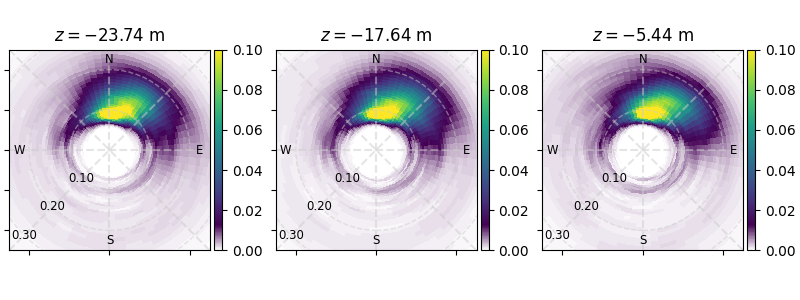
Arrays approach

Now let’s see the array-based approach. First, we need to project the ADCP beam geomtry on the sea surface and then compute the x-y coordinates of each element of the array. For this, we must know the tilt angle (which is generally 25 degrees), the water depth and the location of each beam. I will compute first the x-y-coordinates passing from polar to cartesian coordinates.

# compute beam distribution
tilt_angle = 25
radius = water_depth * np.sin(np.radians(tilt_angle))
# angles = np.array([0, 180, 90, 270, 0])
angles = np.array([180, 0, 90, 270, 0])
radii = np.array([radius, radius, radius, radius, 0])
x = radii * np.cos(np.radians(angles))
y = radii * np.sin(np.radians(angles))

# compute spectra
eta = adcp_dataset["eta"].interpolate_na("time").data.T
spec = ewdm.Arrays.from_numpy(
    time = time,
    surface_elevation = eta,
    position_x = x,
    position_y = y
)
output_array = spec.compute()

Let’s plot array distribution

fig, ax = plt.subplots(1, 1, figsize=(5,5))
for i, (ix, iy) in enumerate(zip(x, y)):
    ax.plot(ix, iy, "o", color="#6145b5", ms=20)
    ax.text(ix, iy, f"{i+1}", color="w", ha="center", va="center")
ax.margins(0.2)
ax.set_xlabel("x [m]")
ax.set_ylabel("y [m]")
ax.set_title("Beam distribution")

Text(0.5, 1.0, 'Beam distribution')

Finally, let’s plot the directional spectra

fig, (ax1, ax2) = plt.subplots(1, 2, figsize=(8,3))
ax1.set_title("Array-based approach")
ax2.set_title(f"Triplet-based $z={-cell_depth:.2f}$ m")

plot_directional_spectrum(
    output_array.directional_spectrum,
    ax=ax1, levels=None, colorbar=True, vmin=0, vmax=0.1,
    axes_kw={"rmin": 0.1, "rmax": 0.35, "rstep": 0.1, "angle": 225},
    cbar_kw={"label": ""}
)
plot_directional_spectrum(
    output_triplets.directional_spectrum,
    ax=ax2, levels=None, colorbar=True, vmin=0, vmax=0.1,
    axes_kw={"rmin": 0.1, "rmax": 0.35, "rstep": 0.1, "angle": 225},
    cbar_kw={"label": ""}
)