Note
Go to the end to download the full example code.
Comparison of different methods
It is a common practice to express the directional wave spectrum, \(E(f,\theta)\), as the product of two functions:
\[E(f,\theta) = S(f) D(f,\theta)\]
where \(S(f)\) is the frequency spectrum and \(D(f,\theta)\) is the directional distribution function. The problem basically consist of finding \(D(f,\theta)\).
This section compares different methods for estimating the directional distribution \(D(f,\theta)\) and the the directional wave spectra \(E(f,\theta)\). We compare the wavelet-based directional method implemented in EWDM with two of the conventional methods based on Fourier spectral analysis, namely Truncated Fourier Series (TSF) and Maximum Entropy Method (MEM).
The results are visualised and compared to understand the performance and differences between these methods.
import numpy as np
import xarray as xr
import scipy.signal as signal

from matplotlib import pyplot as plt

import ewdm
from ewdm.sources import SpotterBuoysDataSource
from ewdm.plots import plot_directional_spectrum

import warnings
warnings.filterwarnings("ignore", category=RuntimeWarning)
Load sample dataset
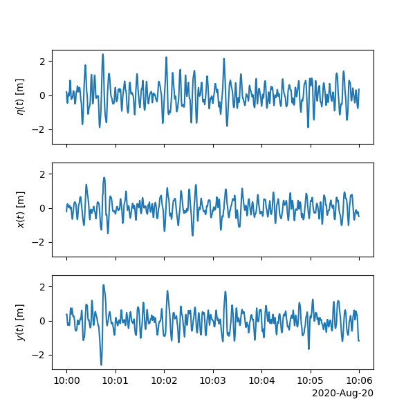
For this example, we use data from a Spotter buoy deployed off the west coast of Ireland in August 2020. In particular, we are using a sample of 30 minutes.
The dataset contains the two horizontal wave-induced displacements and the vertical sea surface elevation.
spotter = SpotterBuoysDataSource("../../data/displacement.csv")
dataset = (
    spotter
    .read_dataset()
    .sel(time=slice("2020-08-20 10:00", "2020-08-20 10:30"))
)
print(dataset)
<xarray.Dataset> Size: 149kB
Dimensions:                 (time: 4650)
Coordinates:
  * time                    (time) datetime64[ns] 37kB 2020-08-20T10:00:00 .....
Data variables:
    eastward_displacement   (time) float64 37kB -0.2063 0.03001 ... -0.1473
    northward_displacement  (time) float64 37kB 0.3724 0.3739 ... 0.08102
    surface_elevation       (time) float64 37kB 0.1855 -0.1143 ... 0.46 0.6334
Attributes:
    sampling_rate:  2.5
Let’s plot a subsample of 5 minutes of these time series to have an idea on what they look like. As it can be seen, the amplitude of the wave-induced buoy movement, in both the horizontal and vertical coordinates, is about 3-4 metres.
# plot time series of the first 5 minutes
fig, (ax1, ax2, ax3) = plt.subplots(
    3,1, figsize=(6,6), sharex=True, sharey=True
)
subset = dataset.sel(time=slice("2020-08-20T10:00", "2020-08-20T10:05"))
subset["surface_elevation"].plot(ax=ax1)
subset["eastward_displacement"].plot(ax=ax2)
subset["northward_displacement"].plot(ax=ax3)
_ = ax1.set(xlabel="", ylabel="$\\eta(t)$ [m]")
_ = ax2.set(xlabel="", ylabel="$x(t)$ [m]")
_ = ax3.set(xlabel="", ylabel="$y(t)$ [m]")
Classic directional spectral analysis
The following class implements the conventional cross-spectral analysis using Fourier transform. This class takes in a dataset containing eastward and northward displacements along with the surface elevation data. The input parameters are sampling frequency of the time series and number of Fourier components for analysis.
Considering the three time series, \(x(t)\), \(y(t)\) and \(z(t)\) (We normally use \(\eta(t)\) for the vertical but it is changed here to \(z(t)\) for simplicity and convenience), the cross-spectral matrix is computed as:
where \(S_{xy}(f)\) is the Fourier cross-spectrum between \(x(t)\) and \(y(t)\), respectively.
Each cross-spectrum can be written in terms of a real (co-spectrum) and an imaginary (quad-spectrum) component:
The auto-spectrum is the cross-spectrum of the same signal, and can be written as \(E_{xx}(f) = S_{xx} S_{xx}^*\), where \(*\) denotes a complex conjugate.
For typical buoy recordings, e.g., three dimensional wave-induced displacements, the circular moments can be written in terms of these auto-, co-, and quad-spectra, like:
See Kuik et al. (1988) and Appendix C in Peláez-Zapata et al. (2024) for further details.
class ClassicSpectralAnalysis(object):
    """This class implements the classic directional spectral analysis"""

    def __init__(self, dataset: xr.Dataset, fs: float=1.0, nperseg=256):
        self.dataset = dataset # time series
        self.fs = fs # sampling frequency
        self.nperseg = nperseg # number of fourier components

    def cross_spectral_matrix(self) -> xr.Dataset:

        # extract variables from dataset
        x, y, z = (
            self.dataset["eastward_displacement"],
            self.dataset["northward_displacement"],
            self.dataset["surface_elevation"]
        )

        # constants
        fft_args = {
            "fs": self.fs,
            "detrend": "constant",
            "nperseg": min(self.nperseg, len(self.dataset["time"])),
        }

        # auto-spectra
        frq, Sxx = signal.welch(x, **fft_args)
        frq, Syy = signal.welch(y, **fft_args)
        frq, Szz = signal.welch(z, **fft_args)

        # cross-spectra
        frq, Sxz = signal.csd(x, z, **fft_args)
        frq, Syz = signal.csd(y, z, **fft_args)
        frq, Sxy = signal.csd(x, y, **fft_args)

        return  xr.Dataset(
            coords = {
                "frequency": ("frequency", frq),
            },
            data_vars = {
                "Sxx": ("frequency", Sxx),
                "Syy": ("frequency", Syy),
                "Szz": ("frequency", Szz),
                "Sxz": ("frequency", Sxz),
                "Syz": ("frequency", Syz),
                "Sxy": ("frequency", Sxy),
            }
        )

    def directional_moments(self, Phi: xr.Dataset) -> xr.Dataset:
        Exx, Eyy, Ezz, Cxy, Qxz, Qyz = (
            np.real(Phi["Sxx"]), np.real(Phi["Syy"]), np.real(Phi["Szz"]),
            np.real(Phi["Sxy"]), np.imag(Phi["Sxz"]), np.imag(Phi["Syz"])
        )

        return  xr.Dataset(
            {
                "a0": Ezz,
                "a1": Qxz / np.sqrt(Ezz * (Exx + Eyy)),
                "b1": Qyz / np.sqrt(Ezz * (Exx + Eyy)),
                "a2": (Exx - Eyy) / (Exx + Eyy),
                "b2": 2 * Cxy / (Exx + Eyy)
            }
        )


csp = ClassicSpectralAnalysis(dataset, fs=dataset.sampling_rate)

# computing the cross-spectral matrix
Phi = csp.cross_spectral_matrix()
print("\nThe cross-spectra matrix is:\n" + 28*"-")
print(Phi)

# computing the directional moments, aka first-five Fourier coefficients
moments = csp.directional_moments(Phi)
print("\nThe circular moments are:\n" + 25*"-")
print(moments)
The cross-spectra matrix is:
----------------------------
<xarray.Dataset> Size: 10kB
Dimensions:    (frequency: 129)
Coordinates:
  * frequency  (frequency) float64 1kB 0.0 0.009766 0.01953 ... 1.23 1.24 1.25
Data variables:
    Sxx        (frequency) float64 1kB 0.007765 0.003491 ... 0.0002501 0.0001311
    Syy        (frequency) float64 1kB 0.01076 0.003956 ... 0.0005091 0.0003085
    Szz        (frequency) float64 1kB 0.01161 0.005453 ... 3.419e-07 3.377e-08
    Sxz        (frequency) complex128 2kB (0.005292409300087139+0j) ... (1.70...
    Syz        (frequency) complex128 2kB (0.004013427745588333+0j) ... (-8.2...
    Sxy        (frequency) complex128 2kB (0.003789505228475266+0j) ... (-4.7...

The circular moments are:
-------------------------
<xarray.Dataset> Size: 6kB
Dimensions:    (frequency: 129)
Coordinates:
  * frequency  (frequency) float64 1kB 0.0 0.009766 0.01953 ... 1.23 1.24 1.25
Data variables:
    a0         (frequency) float64 1kB 0.01161 0.005453 ... 3.419e-07 3.377e-08
    a1         (frequency) float64 1kB 0.0 -0.00558 0.01824 ... 0.08701 0.0
    b1         (frequency) float64 1kB 0.0 0.03565 0.001226 ... -0.2141 0.0
    a2         (frequency) float64 1kB -0.1618 -0.0624 ... -0.3412 -0.4035
    b2         (frequency) float64 1kB 0.409 0.4202 -0.03618 ... -0.2188 -0.2159
Truncated Fourier Series
The most straightforward way of obtaining the directional distribution function \(D(f,\theta)\) is by expanding in Fourier series:
This Fourier series is truncated to \(N=2\) because it is the maximum number of components that can be extracted from buoy measurements.
def tfs_distribution(moments, smoothing=32):
    """Implementation of the Truncated Fourier Series method"""

    dirs =  xr.Variable(dims=("direction"), data=np.arange(-180,180,5))
    D = (1/(2*np.pi)) * (
        1 +
        moments["a1"] * np.cos(np.radians(dirs)) +
        moments["b1"] * np.sin(np.radians(dirs)) +
        moments["a2"] * np.cos(2*np.radians(dirs)) +
        moments["b2"] * np.sin(2*np.radians(dirs))
    )
    D.coords["direction"] = dirs
    D = D.where(D > 0, 0)
    return (
        (D / D.integrate("direction"))
        .rolling(frequency=smoothing, center=True)
        .median()
    )

D_tfs = tfs_distribution(moments, smoothing=2)
print(D_tfs)
<xarray.DataArray (frequency: 129, direction: 72)> Size: 74kB
array([[       nan,        nan,        nan, ...,        nan,        nan,
               nan],
       [0.00250404, 0.00270683, 0.00291287, ..., 0.00197615, 0.00213296,
        0.00231076],
       [0.0019888 , 0.00209034, 0.00221308, ..., 0.00183954, 0.00186136,
        0.00191166],
       ...,
       [0.00174922, 0.00168946, 0.00165851, ..., 0.00205949, 0.00193906,
        0.00183394],
       [0.00167282, 0.00162718, 0.00161289, ..., 0.00196322, 0.00184506,
        0.00174674],
       [0.00163627, 0.00157299, 0.00154485, ..., 0.002007  , 0.00185721,
        0.00173218]], shape=(129, 72))
Coordinates:
  * frequency  (frequency) float64 1kB 0.0 0.009766 0.01953 ... 1.23 1.24 1.25
  * direction  (direction) int64 576B -180 -175 -170 -165 ... 160 165 170 175
Maximum Entropy Method
A more sophisticated way of obtaining the directional distribution function \(D(f,\theta)\) is by using a maximum entropy estimator.
Following Lygre and Krogstad (1983) and Alves and Melo (1999), the form of the directional distribution function can be written as:
where \(c_1\) and \(c_2\) are the complex representation of the Fourier coefficients, i.e.,
and
It is worth noting that this is just one of the possible implementations of MEM. There are other variations that might potentially produce better results. For more details, see Christie (2024) and Simanesew et al. (2018).
def mem_distribution(moments, smoothing=32):
    """Implementation of the Maximum Entropy Method"""

    dirs =  xr.Variable(dims=("direction"), data=np.arange(-180,180,5))

    c1 = moments["a1"] + 1j*moments["b1"]
    c2 = moments["a2"] + 1j*moments["b2"]

    phi1 = (c1 - c2 * c1.conj()) / (1 - np.abs(c1)**2)
    phi2 = c2 - c1.conj() * phi1

    sigma_e = 1 - phi1 * c1.conj() - phi2 * c2.conj()

    D = (1/(2*np.pi)) * np.real(
        sigma_e.expand_dims({"direction": dirs}) /
        np.abs(
            1 - phi1.expand_dims({"direction": dirs}) * np.exp(-1j*dirs*np.pi/180)
              - phi2.expand_dims({"direction": dirs}) * np.exp(-2j*dirs*np.pi/180)
        )**2
    )

    return (
        (D.T / D.integrate("direction"))
        .rolling(frequency=smoothing, center=True)
        .median()
    )

D_mem = mem_distribution(moments, smoothing=2)
print(D_mem)
<xarray.DataArray (frequency: 129, direction: 72)> Size: 74kB
array([[       nan,        nan,        nan, ...,        nan,        nan,
               nan],
       [0.0016726 , 0.00187117, 0.00212643, ..., 0.00130816, 0.00139915,
        0.00151835],
       [0.00136586, 0.00148521, 0.00164393, ..., 0.00118107, 0.00121821,
        0.00127862],
       ...,
       [0.00083521, 0.00080648, 0.00078886, ..., 0.00100139, 0.00093078,
        0.00087611],
       [0.0008874 , 0.00086278, 0.00084955, ..., 0.00104174, 0.0009751 ,
        0.00092435],
       [0.00104805, 0.00101893, 0.00100344, ..., 0.00123452, 0.00115327,
        0.00109213]], shape=(129, 72))
Coordinates:
  * direction  (direction) int64 576B -180 -175 -170 -165 ... 160 165 170 175
  * frequency  (frequency) float64 1kB 0.0 0.009766 0.01953 ... 1.23 1.24 1.25
Wavelet-based directional wave spectrum
Here, we use the ewdm.Triplets module to get an estimation of the directional distribution function \(D(f,\theta)\) using the wavelet-based method applied over the buoy data.
spec = ewdm.Triplets(dataset)
output = spec.compute()
D_ewdm = output["directional_distribution"]
print(D_ewdm)
<xarray.DataArray 'directional_distribution' (frequency: 81, direction: 72)> Size: 47kB
array([[0.00168447, 0.00223245, 0.00297662, ..., 0.00122683, 0.00125593,
        0.00138172],
       [0.00283082, 0.00302224, 0.00295472, ..., 0.00154785, 0.00194835,
        0.00242453],
       [0.00193635, 0.00179175, 0.00167039, ..., 0.00200759, 0.0020642 ,
        0.0020372 ],
       ...,
       [0.00289393, 0.00291756, 0.00293399, ..., 0.00272196, 0.00279641,
        0.00285523],
       [0.00255808, 0.00254595, 0.00258549, ..., 0.00259349, 0.00261379,
        0.00259397],
       [0.0024424 , 0.002416  , 0.00242277, ..., 0.00248775, 0.00250426,
        0.00248145]], shape=(81, 72))
Coordinates:
  * frequency  (frequency) float64 648B 0.03125 0.03263 0.03408 ... 0.9576 1.0
  * direction  (direction) float64 576B -180.0 -175.0 -170.0 ... 170.0 175.0
Attributes:
    standard_name:  sea_surface_wave_directional_distribution_function
    long_name:      Directional distribution function of wave energy
    units:          dimensionless
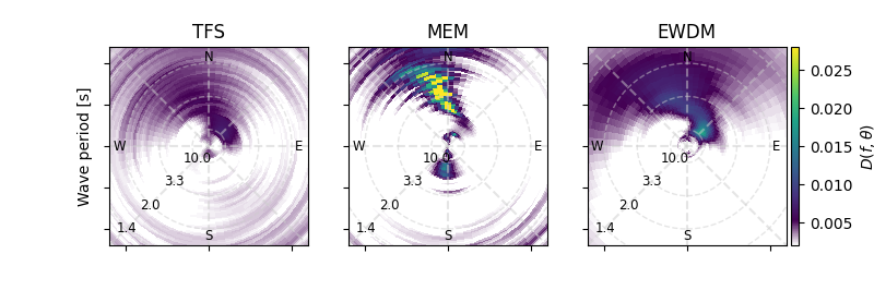
Directional distribution function
The results for the directional distribution function \(D(f,\theta)\) obtained from the three different methods evaluated are shown side-by-side.
vmin, vmax = 0.002, 0.028
axes_kw={"rmax": 0.8, "rstep": 0.2, "as_period": True}

fig, (ax1, ax2, ax3) = plt.subplots(1, 3, figsize=(8,8/3))
plot_directional_spectrum(
    D_tfs, ax=ax1, levels=None, colorbar=False,
    axes_kw=axes_kw, vmin=vmin, vmax=vmax
)
plot_directional_spectrum(
    D_mem, ax=ax2, levels=None, colorbar=False,
    axes_kw=axes_kw, vmin=vmin, vmax=vmax
)
plot_directional_spectrum(
    D_ewdm, ax=ax3, levels=None, colorbar=True,
    cbar_kw={"label": "$D(f,\\theta)$"},
    axes_kw=axes_kw, vmin=vmin, vmax=vmax
)
_ = ax1.set(xlabel="", title="TFS")
_ = ax2.set(xlabel="", ylabel="", title="MEM")
_ = ax3.set(xlabel="", ylabel="", title="EWDM")
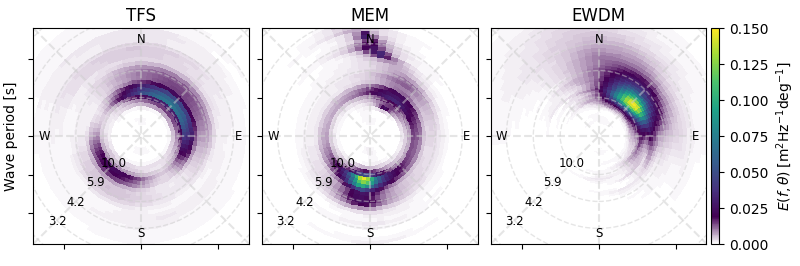
Directional wave spectrum
Now, we show the corresponding directional wave spectra \(E(f,\theta)\) for each method. Recalling that this quantity is constructed as:
For the Fourier-based methods, the frequency spectrum \(S(f)\) is simply the Fourier transform of the surface elevation signal, i.e., \(E_{zz}(f)\), the auto-spectrum of \(z(t)\). For the wavelet method, \(S(f)\) is obtained time-averaging the squared wavelet amplitudes. See Directional distribution and directional spectrum.
# compute the directional wave spectrum
E_tfs = moments["a0"] * D_tfs
E_mem = moments["a0"] * D_mem
E_ewdm = output["directional_spectrum"]

vmin, vmax = 0.0, 0.15
axes_kw={"rmax": 0.35, "rstep": 0.07, "as_period": True}
fig, (ax1, ax2, ax3) = plt.subplots(1, 3, figsize=(8,8/3), layout="constrained")
plot_directional_spectrum(
    E_tfs, ax=ax1, levels=None, colorbar=False,
    axes_kw=axes_kw, vmin=vmin, vmax=vmax
)
plot_directional_spectrum(
    E_mem, ax=ax2, levels=None, colorbar=False,
    axes_kw=axes_kw, vmin=vmin, vmax=vmax
)
plot_directional_spectrum(
    E_ewdm, ax=ax3, levels=None, colorbar=True,
    cbar_kw={"label": "$E(f,\\theta)\\;\\mathrm{[m^2 Hz^{-1} deg^{-1}]}$"},
    axes_kw=axes_kw, vmin=vmin, vmax=vmax
)
_ = ax1.set(xlabel="", title="TFS")
_ = ax2.set(xlabel="", ylabel="", title="MEM")
_ = ax3.set(xlabel="", ylabel="", title="EWDM")
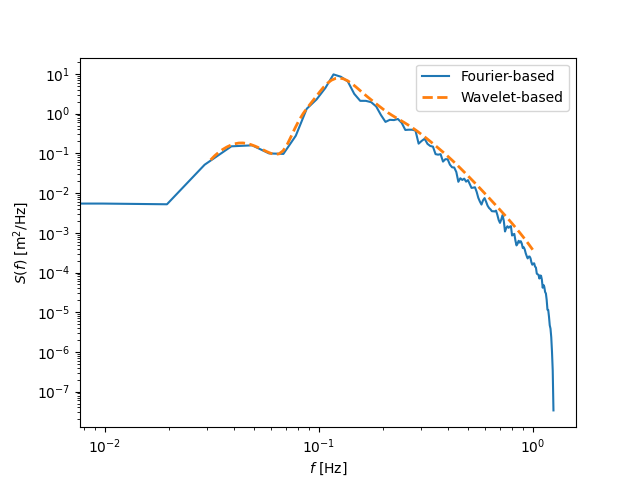
Azimutally-integrated power spectrum
A quick comparison between azimutally-integrated wavelet power and Fourier-based power density spectrum, \(S(f)\), is presented.
This comparison reveals similarities. The wavelet spectrum inherently offers lower frequency resolution compared to the Fourier spectrum, thus resulting in a naturally smoother representation of the energy distribution. This characteristic of the continuous wavelet transform has been extensively discussed. See e.g., Torrence and Compo (1998).
fig, ax = plt.subplots()
ax.loglog(moments["frequency"], moments["a0"], label="Fourier-based")
output.frequency_spectrum.plot(ax=ax, ls="--", lw=2, label="Wavelet-based")
ax.set(xlabel="$f$ [Hz]", ylabel="$S(f)$ [m$^2$/Hz]")
ax.legend()
<matplotlib.legend.Legend object at 0x7e1d6c03b340>
Discussion and conclusion
The comparison of three methods for estimating the directional wave spectrum reveals distinct characteristics:
TFS is too broad, i.e., it spreads too much the energy across the directions, which is inconsistent with previous observations.
MEM seems to be too narrow and shows spurious peaks. In addition, it tends to produce inconsistent bimodal distributions. For example, it identifies waves travelling south which appear to e unrealistic.
EWDM results appear consistent showing a smooth transition of wave energy across frequencies and directions.
However, objectively evaluating the quality of these estimations is challenging due to the lack of a ground truth reference. Consequently, further research is imperative to enhance the understanding and assessment of these methods. Despite this limitation, EWDM exhibits promise in providing more reliable estimates for the directional wave spectrum.
Total running time of the script: (0 minutes 1.338 seconds)