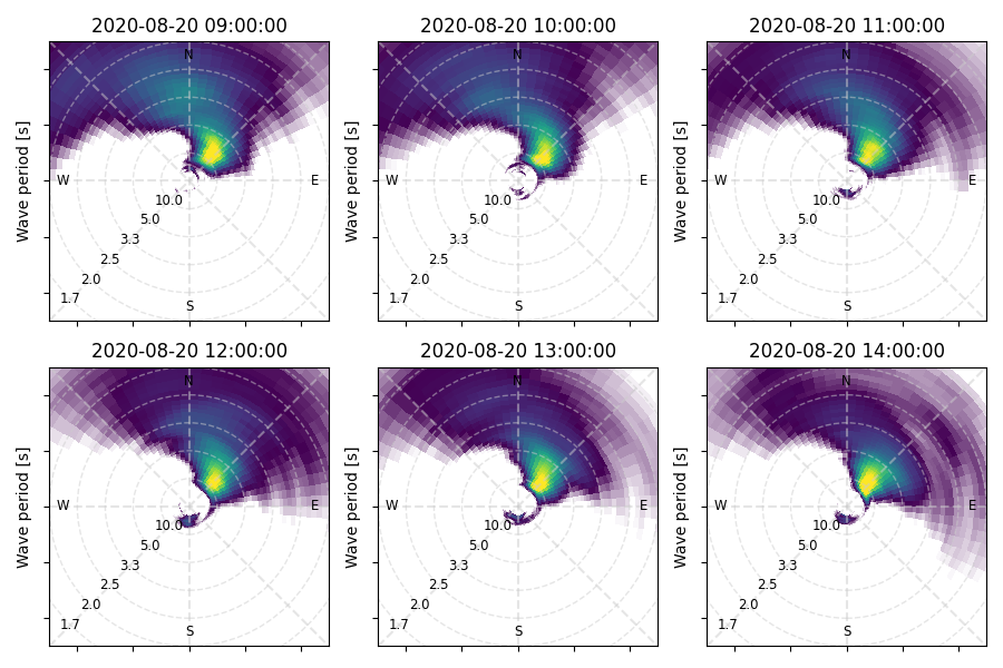
Using Spotter buoy data

In this example we demostrate how to use ewdm package to compute directional wave spectrum from Spotter buoy data. In particular, we use the displacement.csv file that is generated after running the parsing script provided by SOFAR. This file containes time series of surface elevation and wave displacements.

We also show that for datasets with more than one hour of data, the wave spectra are computed over blocks of 30 minutes (by default).

Processing::   0%|          | 0/6 [00:00<?, ?it/s]
Processing::  17%|█▋        | 1/6 [00:00<00:03,  1.30it/s]
Processing::  33%|███▎      | 2/6 [00:01<00:03,  1.32it/s]
Processing::  50%|█████     | 3/6 [00:02<00:02,  1.32it/s]
Processing::  67%|██████▋   | 4/6 [00:03<00:01,  1.32it/s]
Processing::  83%|████████▎ | 5/6 [00:03<00:00,  1.33it/s]
Processing:: 100%|██████████| 6/6 [00:04<00:00,  1.33it/s]
Processing:: 100%|██████████| 6/6 [00:04<00:00,  1.32it/s]

import numpy as np
import xarray as xr

from matplotlib import pyplot as plt

import ewdm
from ewdm.sources import SpotterBuoysDataSource
from ewdm.plots import plot_directional_spectrum

spotter = SpotterBuoysDataSource("../../data/displacement.csv")
dataset = spotter.read_dataset()
spec = ewdm.Triplets(dataset)
output = spec.compute(
    omin=-5, omax=0, nvoice=16, dd=5, kappa=36,
    block_size="60min", use="displacements"
)

fig, axs = plt.subplots(2, 3, figsize=(9,6), layout="tight")
axs = axs.ravel()
for ax, tt in zip(axs, output.time):
    plot_directional_spectrum(
        output.sel(time=tt).directional_distribution,
        ax=ax, vmin=0.003, vmax=0.015, levels=None, colorbar=False,
        axes_kw={"rmax": 0.6, "as_period": True}
    )
    ax.set_title(tt.dt.strftime("%Y-%m-%d %H:%M:%S").item())