Donelan run82 test case

This example shows ewdm.Arrays in action. We use the run82 as test case. More information about this test case can be found in Donelan et al. 2015

import numpy as np
import xarray as xr

from scipy.io import loadmat
from matplotlib import pyplot as plt

import ewdm
from ewdm.plots import plot_directional_spectrum

# loading matlab file
mat_fname = "../../data/donelan_run82.mat"
mat_data = loadmat(mat_fname, simplify_cells=True)

sampling_rate = mat_data["fs"]
time = np.arange(len(mat_data["eta"])) / sampling_rate
elements = np.arange(len(mat_data["x"]))

# creating dataset
dataset = xr.Dataset(
    data_vars = {
        "surface_elevation": (["time", "element"], mat_data["eta"]),
        "position_x": ("element", mat_data["x"]),
        "position_y": ("element", mat_data["y"])
    },
    coords = {"time": time, "element": elements},
    attrs = {"sampling_rate": sampling_rate}
)
print(dataset)

<xarray.Dataset> Size: 230kB
Dimensions:            (time: 4096, element: 6)
Coordinates:
  * time               (time) float64 33kB 0.0 0.25 0.5 ... 1.024e+03 1.024e+03
  * element            (element) int64 48B 0 1 2 3 4 5
Data variables:
    surface_elevation  (time, element) float64 197kB 0.02559 0.03397 ... 0.08992
    position_x         (element) float64 48B 0.0 0.2097 ... -0.08959 0.1943
    position_y         (element) float64 48B 0.0 0.1362 ... -0.2334 -0.1573
Attributes:
    sampling_rate:  4

Let’s first have a look at the array configuration

fig, ax = plt.subplots()
ax.scatter(dataset["position_x"], dataset["position_y"], s=500, c="k")
for element in dataset["element"]:
    ax.text(
        dataset["position_x"].sel(element=element).item(),
        dataset["position_y"].sel(element=element).item(),
        element.item(), ha="center", va="center", color="w"
    )
ax.set_aspect('equal', adjustable='box')
ax.set(title="Array geometry", xlabel="x [m]", ylabel="y [m]")
print(f"Number of elements in the array: {len(dataset['element'])}")

Number of elements in the array: 6

Let’s compute the directional spectrum

spec = ewdm.Arrays(dataset)
output = spec.compute(
    cross_wavelet=True, solver="least-squares", kappa=36
)
print(output)

<xarray.Dataset> Size: 114kB
Dimensions:                   (frequency: 97, direction: 72)
Coordinates:
  * frequency                 (frequency) float64 776B 0.03125 0.03263 ... 2.0
  * direction                 (direction) float64 576B -180.0 -175.0 ... 175.0
Data variables:
    directional_spectrum      (frequency, direction) float64 56kB 1.565e-06 ....
    directional_distribution  (frequency, direction) float64 56kB 0.004159 .....
    frequency_spectrum        (frequency) float64 776B 0.0003762 ... 3.766e-05

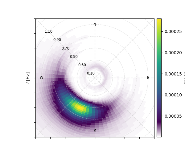
Now let’s plot the output. Here we can tune up the plot_directional_spectrum function. For example, let’s start radius ticks from 0.1 to 1.2 Hz every 0.2 Hz. Also, let’s rotate them 135 degrees (northwest). Finally, let’s add a colorbar label.

fig, ax = plt.subplots(figsize=(6,5))
plot_directional_spectrum(
    output.directional_spectrum, ax=ax, levels=None, colorbar=True,
    axes_kw={"rmin": 0.1, "rmax": 1.2, "rstep": 0.2, "angle": 135},
    cbar_kw={"label": "$E(f,\\theta)$"}
)