Estimating directional spectra from stereo-imaging

Stereo-imaging has emerged as a unique measurement technique for obtaining precise directional information about wave fields. One of its key advantages lies in the direct estimation of directional wave spectra through three-dimensional Fourier analysis.

The quality of the directional spectrum is intricately tied to the resolution of the images captured. Higher image resolution can provide insights into small-scale wave features, including the dynamics of growing waves and wave-breaking processes.

However, large-scale wave features, such as long waves (e.g., swell), may fall beyond the camera’s field of view. In such cases, alternative techniques may need to be considered. For example, one approach involves selecting several pixels from the image and extracting the time series of the surface elevation. This can then be used to construct the directional spectrum from the data.

This example uses data from Guimaraes et al (2020) taken at the Black Sea. We explore different results changing the number and distribution of pixels in the image.

import numpy as np
import xarray as xr
import netCDF4 as nc
import matplotlib.pyplot as plt
import matplotlib.image as mpimg
import urllib.request
import subprocess
import os

from scipy.io import loadmat

import ewdm
from ewdm.plots import plot_directional_spectrum

# define paths and filenames
URL = "https://data-dataref.ifremer.fr/stereo/BS_2013/"
VIDEO_URL = URL + "2013-09-22_13-00-01_10Hz/nc/Surfaces_20130922_130001_short.nc"
IMAGE_RIGHT_URL = URL + "2013-09-22_13-00-01_10Hz/input/000111_01.tif"
IMAGE_LEFT_URL = URL + "2013-09-22_13-00-01_10Hz/input/000111_02.tif"
CACHE_DIR = "../../data/"
LOCAL_VIDEO_FILE = os.path.join(CACHE_DIR, "stereo-video.nc")

Exploring stereo-video dataset

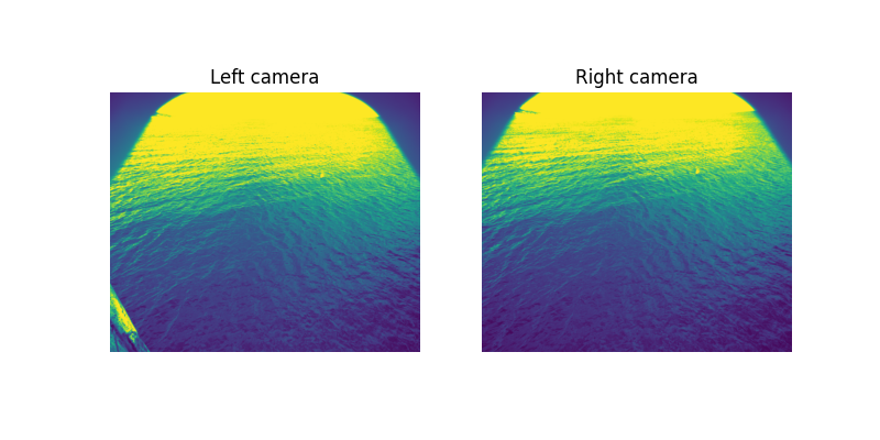
First, let’s see what a typical stereo-image looks like. Below, the first frame of the Black Sea data is shown.

# load images
img_right = mpimg.imread(urllib.request.urlopen(IMAGE_RIGHT_URL), format='tif')
img_left = mpimg.imread(urllib.request.urlopen(IMAGE_LEFT_URL), format='tif')

# plot images
fig, (ax1, ax2) = plt.subplots(1, 2, figsize=(8,4))
ax1.imshow(img_left)
ax2.imshow(img_right)
ax1.axis('off')
ax2.axis('off')
ax1.set_title("Left camera")
ax2.set_title("Right camera")
plt.show()

Computing directional wave spectra

Now, we are going to download the netCDF4 containing the streo-images data and place it into the data folder. This might take a few minutes.

# check if the file is already cached
if not os.path.exists(LOCAL_VIDEO_FILE):
    print("Downloading the stereo-video file. It might take a few minutes.")
    command = f"wget {VIDEO_URL} -O {LOCAL_VIDEO_FILE}"
    subprocess.call(command, shell=True)
else:
    print("File already exists. Skipping download.")

# laod the video data as netcdf
nc_obj = nc.Dataset(LOCAL_VIDEO_FILE)

Downloading the stereo-video file. It might take a few minutes.

To pick the pixels, we define the corresponding indices. We are going to evaluate four different configurations.

1. The optimal array proposed by Young et al (1994).

2. A simple pentagon.

3. 10 random points.

4. 20 random points.

indices1 = [
    (95,95), (95,175), (95,15), (175,15), (15,15),
    (115,95), (75,95), (95,75)
]
indices2 = [
    (95,95), (95, 5), (171, 62), (138, 161), (55, 161), (22, 62)
]
indices3 = [tuple(np.random.randint(40, 150, size=2)) for _ in range(10)]
indices4 = [tuple(np.random.randint(40, 150, size=2)) for _ in range(20)]
titles = ["Young (1994)", "Pentagon", "10 random", "20 random"]

# loop for each configuration
for indices, title in zip((indices1, indices2, indices3, indices4), titles):

    # pick the elevation time series from the image
    x = np.array([nc_obj["X"][i,j] for i,j in indices])
    y = np.array([nc_obj["Y"][i,j] for i,j in indices])
    eta = np.array([nc_obj["Z"][:8192,i,j] for i,j in indices])
    time = nc.num2date(nc_obj['time'][:8192], units=nc_obj["time"].units)
    elements = np.arange(len(x))

    # create input dataset
    dataset = xr.Dataset(
        data_vars = {
            "surface_elevation": (["time", "element"], eta.T),
            "position_x": ("element", x),
            "position_y": ("element", y)
        },
        coords = {"time": time, "element": elements},
        attrs = {"sampling_rate": 10}
    )

    # run the ewdm.Arrays code and obtain the directional spectrum
    spec = ewdm.Arrays(dataset)
    output = spec.compute(
        cross_wavelet=True, solver="least-squares", kappa=36
    )

    # plot the results
    fig, (ax1, ax2) = plt.subplots(1, 2, figsize=(8,3.5))
    plot_directional_spectrum(
        output.directional_spectrum, ax=ax2, levels=None, colorbar=True,
        axes_kw={"rmin": 0.1, "rmax": 1.2, "rstep": 0.2, "angle": 135},
        cbar_kw={"label": "$E(f,\\theta)$"}
    )
    ax1.pcolormesh(
        nc_obj["X"][:,:], nc_obj["Y"][:,:], nc_obj["Z"][0,:,:],
        cmap="bwr", vmin=-0.5, vmax=0.5
    )
    ax1.plot(x, y, "o", mec="indigo", mfc="w")
    ax1.set_title(title)

• 
• 
• 
• 

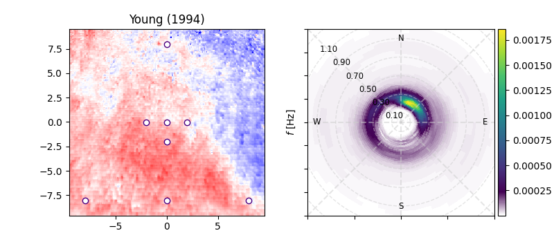
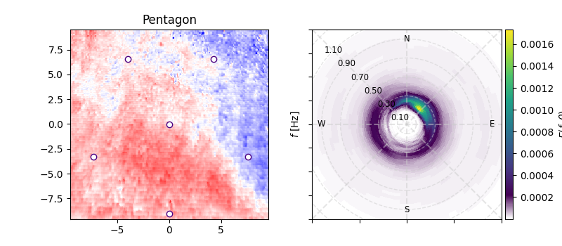
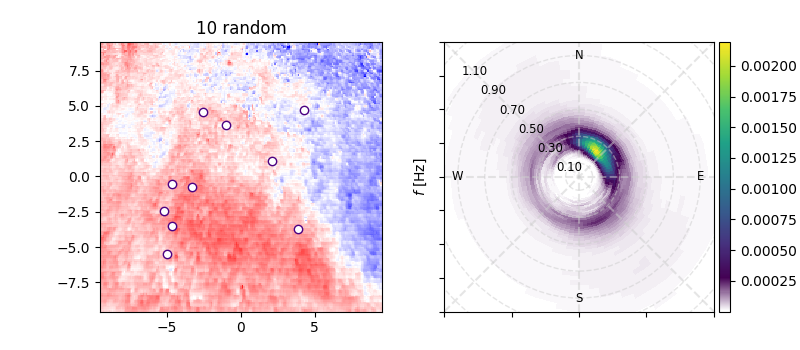
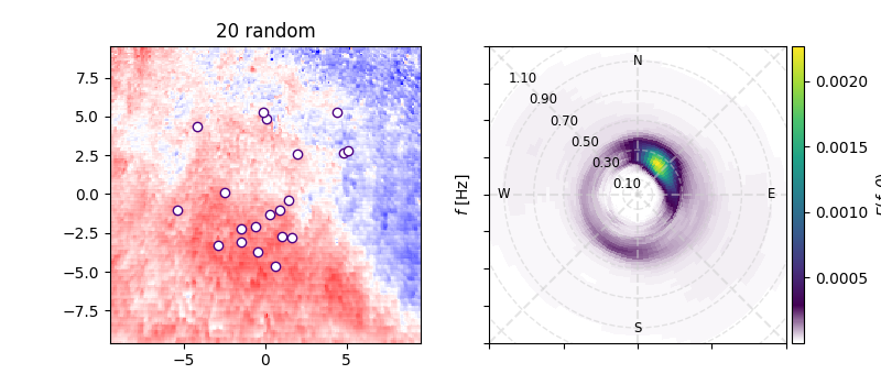
There are clearly some differences between the chosen configurations. The overal quality of the directional spectrum depends on the array distribution. However, we confirm that the main wave direction obtained in all cases is consistent with the reported by Guimaraes et al (2020).